BI Guiding - Understanding time series forecast with smart predict

The aim of this blog post is to in a simple way explain the underlaying mechanisms which Time series forecasting in SAP Analytics Cloud is built upon. We will explore the mathematical ideas and the number-crunching that allows Smart Predict to estimate everything from fashion trends to your company’s future revenue.

This is the third in a series of blog posts on Smart Predict, starting with ‘Understanding Regression with Smart Predict’ and ‘Understanding Classification with Smart Predict’. Time Series Analysis (TSA) is not as similar to Classification and Regression as they are to each other, so this blog can be read and understood on its own.

The point of Time Series Analysis

What we ultimately hope to achieve with TSA is a reliable prediction of the value of a numerical variable (which we shall call the signal) at timepoints in the future. This means Time Series Analysis deals with extrapolation by identifying the signal in the future based on past data points. If we have knowledge of some other variables (so-called candidate influencers), which we have reason to believe could affect the signal, TSA allows us to take these into account as well. For example, TSA can help us answer such questions as:

How many sales can I expect this salesman to close each month of next year?
How many cargo trucks will we need tomorrow if we expand our marketing?
What will my revenue be in my ice-cream shop next month if the weather is good and there are 4 weekends that month?

I have highlighted the signals in bold and the candidate influencers in italics. Note that we can have time and any other number of candidate influencers as we like. Time is a mandatory influence for TSA which is why it is set as a mandatory Data Variable in SAC, but since the mathematical principles are the same, for ease of understanding it will be described as a candidate influence

The signal needs to be a numerical variable (a measure), whereas the candidate influencers can be both dimensions and measures.

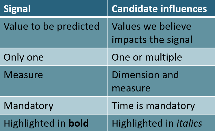
Figure 1: Differences between a signal and candidate influences used for Time Series Analysis

The Idea Behind Time Series Analysis

A note for those familiar with regression. The setup for Time Series Analysis is not dissimilar to that of regression: we want to predict a numerical variable based on a set of influencer variables. But for Time Series Analysis we require one of these candidate influencer variables to be ‘time’, and we put extra emphasis on this variable. The method is tailored specifically to problems in which time is the most important factor in determining the target value/signal. For example, we know that many signals behave cyclically over time (especially in business settings, because of such concepts as seasonality), which our regular regression algorithm is not very good at handling; but as we shall see, Time Series Analysis very actively tries to model this cyclic behavior.

Our predictions will be based on analyzing the behavior of the signal in the past and extrapolating that behavior into the future. To do so we will need to know the values of the signal at some discrete previous times. For simplicity we just write these times as t = 1, t = 2 up to the most recent timepoint, t = N. The timepoints may have any unit, and the distance between each of them is known as the time granularity of our data.

Let us denote the true signal not distorted by noise at time t by y(t). We will aim to find a model, f, which, if it had been applied in the past, would have been efficient at predicting the not-quite-as-distant past. More formally, if it had been applied at time t₀ (when only y(1), y(2), …, y(t₀) was known), it would have made good predictions for the next time points:

Where H is the number of time steps we want to predict.

If we find such a model – that would have ‘worked’ if it were applied in the past – it seems reasonable to believe that it will also ‘work’ now and in the near future. This is the fundamental idea at work in all supervised machine learning.

Throwing stuff against the wall and seeing what sticks

SAC Time Series Forecasts takes a wonderfully simple approach to finding a good predictive model: Try a bunch of different models and pick the one that works the best. This blog post does not concern itself too much with how these different models are individually optimized; instead, I hope to give you a good intuition for what they look like, and what this means for the predictions that they make.

There are two main categories of models:

Trend/Candidate Influencers/Cycle/Fluctuation decomposition
Exponential smoothing

Trend/Candidate Influencers/Cycle/Fluctuation decomposition

Figure 2: The decomposition steps used for understanding the signal to create a machine learning model

The idea here is to split the signal into three or four components: Trend, Candidate Influencers, Cycle and Fluctuation. Which we will go into one at a time.

Trend

First, a general trend is determined to model the overall behavior of the signal. The algorithm tries out 4 possible trends.

Trend 1: Affine function of time

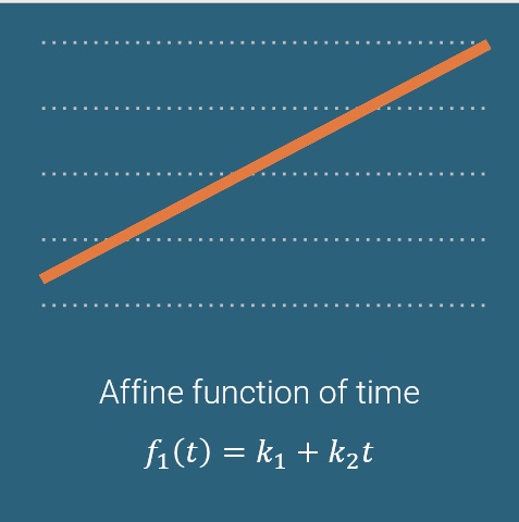
Figure 3: A simpl e linear example of using time to understand the trend for a signal

This function only use the time, t, to calculate the trend. Since it is a function of one variable, it is plotted in 2D; I have plotted it for some choice value of the coefficients k₁ and k₂. With real signal data, the optimal coefficients (chosen so that the trend describes the signal in the past as well as possible) are used.

Trend 2: Lag-1 repetition of the true signal

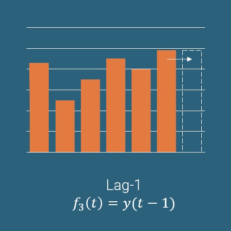
Figure 4: Examples of copying result from previous data points to predict the trend for a signal

This model uses the most recent data point in the true known signal, y, and repeats it.

Trend 3: Linear combination of candidate influencers

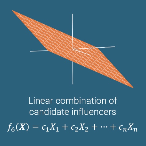
Figure 5: Example of predicting the trend only using candidate influencers

This function calculates the trend only from the optional candidate influencers (which can be stored in a vector X) and completely ignores the time. Once again, the coefficients (c1, …, cn) are chosen to optimize how well the model describes the known data. I have illustrated the function in the case of just two candidate influencers, in which the graph is a plane.

Trend 4: Combination of trend 1 and 3

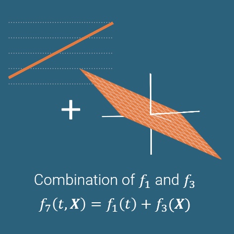
Figure 6: Example of predicting the trend using candidate influencers and time

These function combine the candidate influence of time and two other influences stored in a vector X.

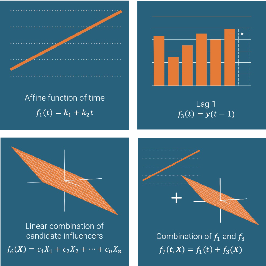
Figure 7: Combined overviewed of ways SAP Analytics Cloud predicts the trend for a signal

SAC has also added the option of following different trends in different time intervals, yielding a piecewise function.

We optimize a model using each of these trends individually, and (so far) won’t discard any of them. Each of them is passed on to the next step in the trend/candidate influencers/cycle/fluctuation-decomposition.

Cycle

For each trend, f, we calculate the remainder, r, of the signal once the trend is removed: r(t) = y(t) – f(t). Then we try to describe this remainder using a cyclic function, i.e., a function which repeats itself. In particular, the following cycles are tested:

Periodic functions: A function c is called n-periodic if it repeats itself every n timesteps, so that c(t) = c(t ± n) = c(t ± 2n) = ….

Figure 8: Visualization for part of a 4-periodic function

Smart Predict tries out periods from n = 1, n = 2 up to n = N/12, where N is the total number of training timepoints (although if N/12 is very large, Smart Predict limits itself to a maximum of n = 450).
For a specific timepoint t₀, the value of c(t₀) = c(t₀ ± n) = c(t₀ ± 2n) = … is chosen as the average of those values it should approximate: the average of r(t₀), r(t₀ + n), r(t₀ – n), r(t₀ + 2n), r(t₀ – 2n) etc. (for all those timepoints where we know the value of r(t)).

Seasonal cycles: Smart Predict also tests cycles that are not periodic in the mathematical sense, but are instead periodic in the human calendar. For example, if we have signal measurements every day throughout several years, we might find that r(t) is approximately the same all of January and that it is the same again next January (and that the same holds true for the other months). Then we would say that the signal had a cycle duration of 1 year and a cycle time granularity of 1 month.
As before, the value of the cyclic function c at time t₀ would be calculated as the average of all the values it should approximate: if t₀ is in January, c(t₀) would be the average of r(t) for all measurements in January.
The possible seasonal cycles that can be found are:

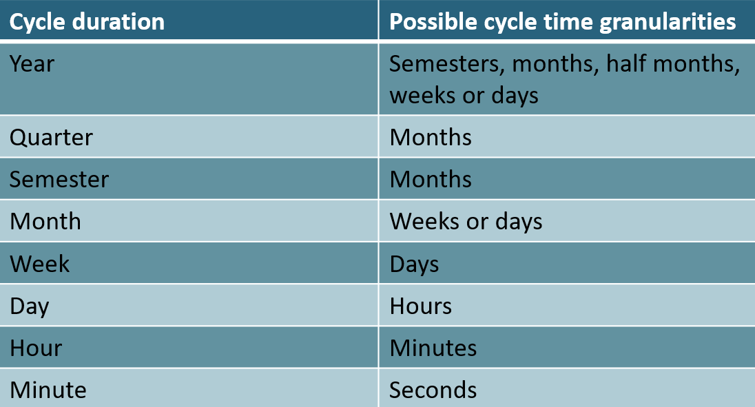
Figure 9: Table of seasonal cycles and possible granularities

Once we have found a cycle which improves how closely the predicted signal matches the true signal, we can try to calculate the remainder again and describe that using another cycle. This process can be repeated for as long as the model improves. More formally, a branch-and-bound algorithm is used to find the best combination of cycles to add for each trend:

Use the trend f_i(t) as our current model, g(t)
Store g(t) as the best model based on trend i we have seen so far, G_i(t) = g(t)
Calculate the remainder r(t) = y(t) – g(t)
Assume that g(t) cannot be improved by adding a cycle on top: improvable = False
For every possible cycle c(t) as described above:
If g(t) + c(t) describes the signal y(t) better than only g(t) did:
Store the fact that g(t) could be improved: improvable = True
Recursively repeat line 3-10 using g(t) + c(t) instead of g(t)
If improvable = False (if g(t) is as good as it can become along this branch)
Check if g(t) is better than G_i(t). If it is, replace G_i(t) by g(t).

Running this algorithm for each i from 1 to 2 yields 2 new functions, G_i(t), which are passed on to the next step in the trend/candidate influencers/cycle/fluctuation decomposition.

Fluctuation

For each ‘trend + cycle’-option, G(t), we once again calculate the remaining signal, s(t), which is s(t) = y(t) – G(t). We then attempt to describe the remainder by an autoregressive (AR) model, a type of function which (like Lag1, Lag2 and double differencing) directly uses the previous values to predict future values; so if, for example, additional sales cause further additional sales, an AR model will be good at describing that.

The AR model is defined by:

where p is known as the order of the model. In the case of Time Series Analysis in Smart Predict this is a maximum of 2 to streamline the analysis and interpretation. We choose the coefficients ci by requiring that the model would have produced good results at all times in the past where it can be evaluated and compared with the true signal:

In particular, we use the least squares method, meaning that we want the sum of the squares of the errors at each time point to be as small as possible:

Since AR is linear, minimizing this loss function is perhaps the most fundamental task in all of optimization, and it is easily done by solving something called the normal equations.

Exponential smoothing

In a sense, this model also splits the signal into three components, but their interaction is different.

Figure 10: The steps for creating a machine learning model using exponential smoothing

Much like the trend/candidate influencers /cycle/fluctuation-decomposition, exponential smoothing actively models periodicity in the signal, but it does so by multiplying a periodic component rather than adding a cycle . Where the trend/candidate influencers/candidate influencers/cycle/fluctuation-decomposition might discover that sales grow by 100.000 units every December, exponential smoothing can discover that sales grow by 10% every December.

Exponential smoothing also puts more weight on the newest data, so you can argue that it adapts more quickly to new behaviour of the signal.

Simple exponential smoothing

We replace our signal y by a smoothed version l. l is meant to describe the general “level” of the signal after some noise has been filtered out. Once we know the level at the latest time point, t = N, we can use it as our prediction into the future (yielding a constant prediction, so clearly this is a very simplistic model). We can write this as:

Where the left-hand-side should be read “the estimate of y(N + h) if we know y until time N”.

But how do we determine the level? At every discrete timepoint t, it is governed by this equation:

For some α between 0 and 1 (we will sometimes use square brackets as arithmetic parentheses to make reading easier). So the level is always calculated as a weighted average of the true signal and the previous level. α describes how little smoothing should be done (at α = 1, we do no smoothing since l(t) = y(t); at α = 0 we have a completely smoothed/constant signal since l(t) = l(t – 1)).

Note that using the smoothing-equation k times yields:

So we multiply the previous signal value y(t–h) by (1-α)^h, making it exponentially less important the further ago it is – hence the name exponential smoothing.

The equation above also exposes the fact that we need l(0) to calculate l at all later times.

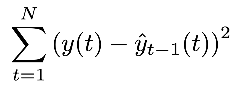
Like always, we will pick our parameters (here l(0) and α) such that the model would have performed as well as possible if it had been used in the past. We will use the least squares method and predict just a single step into the future, so we will minimize

Double exponential smoothing

In addition to the level, we will now add a slope, s, which models the change in the signal from one timepoint to the next. The resulting model is described by these three equations:

For some α, β between 0 and 1.

The slope should model the change l(t) – l(t-1), but is smoothed using a weighted average, just like we did for the level.

The prediction now includes the slope. After the last known timepoint, we assume that the slope remains constant, so after h timesteps, the signal has grown hs(N) from where it started at l(N).

The level has been adjusted slightly. Like before, it is a weighted average of the true signal y(t) and our best estimate of y(t), which is ŷ_t_-1(t) – but since we have updated the formula for ŷ_t_-1(t), we have also updated the formula for l.

Now α, β, l(0) and s(0) are all determined by least squares.

Triple exponential smoothing

The last component we add to our model is a periodicity.

For some α, β, γ between 0 and 1, and for a period m.

The prediction is now multiplied by a periodic factor p(t’), where t’ is a timepoint in the period immediately before N, placed at the same point during the period as N+h is in its period for example, assume that:

the time granularity is “months”
m = 12 (so the period is a year)
N corresponds to December 2022
N+h corresponds to October 2024

Then t’ corresponds to October 2022.

The periodic factor should describe the ‘boosting power’ (or the decreasing power) of a certain time during the period, such as a certain month. If we take the general level, l, and multiply by the boosting power, we should get the true signal, so we want l(t)·p(t) ≈ y(t) ⇔ p(t) ≈ y(t)/l(t).

This fraction is present in the final formula for p(t), but we can get a better estimate of the ‘power’, by also taking into account how much the signal was boosted at the same in the previous periods (at times t–m, t-2m etc.). The longer ago, the less important, so we reemploy the “exponential smoothing”-average that we have come to know and love.

The level should now describe the general level of the signal before the boost from the periodic factor, so we divide the true signal by p(t–m) before we use it in the calculation. We cannot divide by p(t) since we need to calculate the level before the periodicity; p(t–m) is the best substitute.

The slope is unchanged

Now α, β, γ, l(0), s(0) and p(0) are all determined by least squares.

For your convenience, this figure sums up exponential smoothing:

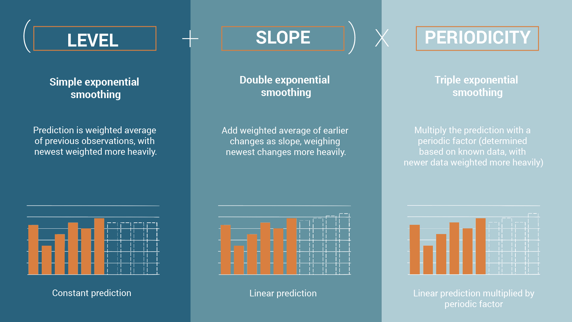
Figure 11: Exponential Smoothing for identifying a signal

But what model is my time series forecast based on?

In the explanation tab of a time series forecast, SAP Analytics Cloud helps you to understand what model has been used.

If a trend/cycle/fluctuation-decomposition has been used

The Time Series Breakdown will feature the following text:

“The predictive model was built by breaking down the time series into basic components”

A plot will show you both the trend (split into time-dependent and influencer-dependent parts), the cycle and the fluctuation.

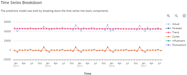
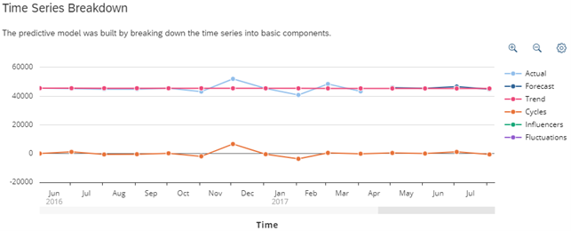
Figure 12: Explanation for a predictive model in SAP Analytics Cloud if trend/candidate influencer/cycle/fluctuation decomposition was used for the model

Note that the model only begins ‘working’ after 3 timesteps; this is because the AR model used for the fluctuation component is of order 2, so it relies on the previous 2 signal values.

Quite often (as is the case here), no influencers are present in the final model, because they are not used in the trend that ends up being used. In some cases, no fluctuations are present, because adding an AR model does not significantly improve the final model.

You will also get an overview of how much impact each component had, given as a percentage of the overall impact.

Figure 13: Overview of the impact for each trend/candidate influencers/cycle/fluctuation decomposition component used for the model

The final residuals are the parts of the signal that the model was not able to explain.

The vast majority of the impact is almost always attributed to the trend, since it is responsible for the overall level of the signal. Even though the impact of the trend is overwhelming, the business user may get more information/insight from the cycles and/or fluctuations.

Finally, there is a nice explanation of what kind of trend and cycle has been used:

Trend 1 “Affine function of time” was used

The cycle duration was 1 year

The AR model is of order 0 meaning the remainder of the signal after the trend and cycles was analyzed had no significant impact on the forecasting.

If exponential smoothing has been used

The Time Series Breakdown now states:

“The predictive model was built incrementally by smoothing the time series, with more weight given to recent observations”

And the plot shows the trend (the level + slope component) and the cycles (the impact of the periodicity):

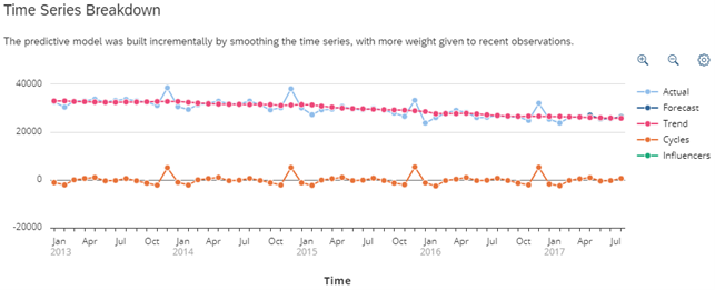
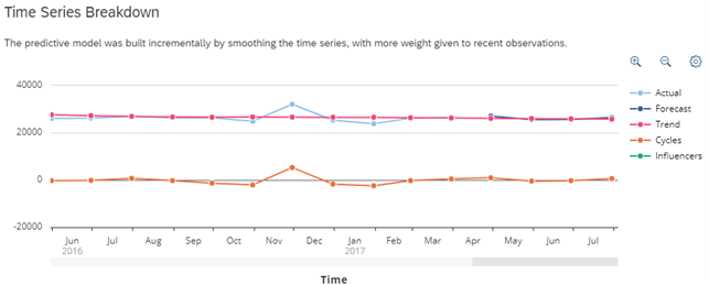
Figure 15: Explanation for a predictive model in SAP Analytics Cloud if exponential smoothing was used for the model

Exponential smoothing also comes with an explanation regarding the impact of each component, and a description regarding the trend and cycles, where the trend will state:
“The Time series doesn’t follow any simple trend, a data smoothing technique was used to estimate a linear trend for the forecase”

But what is the accuracy of my model?

To find the accuracy of your forecasting model go into the Overview tab and look for the MAPE. MAPE (Mean Absolute Percentage Error) gives the absolute percentage difference between the actual and forecasted values, meaning the lower the percentage the better the model was to predict known values of the signal. The way Smart Predict does this is by only taking 75% of the input data to create the model and the remaining 25% to test its accuracy. It is also this way that Smart Predict chooses the most accurate model to present.

A LEAN predictive planning future

Looking at the official future roadmap for Smart Predict in SAP Analytics Cloud, lots of emphasis is on enabling users to get additional insights and build more trust in their Time Series Analyses. This can be seen in their 2023 January LEAN update. Smart Predict is truly developed for and is continuously being updated to enable the general user to do advanced machine learning for their planning purposes in an easy manner to do and understand.

Conclusion

Time Series Forecasting when critically understood, is a worthwhile option for financial forecasting and planning. I hope this post helped in understanding the underlying model used for Smart Predict in SAP Analytics Cloud.

Cookie	Duration	Description
cookielawinfo-checkbox-analytics	11 months	This cookie is set by GDPR Cookie Consent plugin. The cookie is used to store the user consent for the cookies in the category "Analytics".
cookielawinfo-checkbox-functional	11 months	The cookie is set by GDPR cookie consent to record the user consent for the cookies in the category "Functional".
cookielawinfo-checkbox-necessary	11 months	This cookie is set by GDPR Cookie Consent plugin. The cookies is used to store the user consent for the cookies in the category "Necessary".
cookielawinfo-checkbox-others	11 months	This cookie is set by GDPR Cookie Consent plugin. The cookie is used to store the user consent for the cookies in the category "Other.
cookielawinfo-checkbox-performance	11 months	This cookie is set by GDPR Cookie Consent plugin. The cookie is used to store the user consent for the cookies in the category "Performance".
viewed_cookie_policy	11 months	The cookie is set by the GDPR Cookie Consent plugin and is used to store whether or not user has consented to the use of cookies. It does not store any personal data.

Understanding time series forecasts with smart predict