understanding regression with smart predict

This blog post will provide insight into the inner workings of the regression algorithm in SAC Smart Predict. The goal is to help you gain an intuitive understanding of what goes on under the hood, so that you can better evaluate and make informed decisions about the models that you train.

The Point of Regression

In a predictive context, the goal of regression is to predict the value of a numerical variable based on the known values of some influencer variables. For example, regression can help us answer such questions as:

• “How many units will my new factory be able to produce?”
• “How expensive should this customer’s health insurance be?”
• “How much interest will my product garner in a new market?”

Note that influencer variables can be both dimensions (nominal variables such as whether an insurance customer smokes) and measures (numerical variables such as the square footage of a factory). A general mathematical framework for regression is thus:

We want to predict a measure y from influencer variables x₁, x₂, …, x_m, each of which can be either measures or dimensions.

The Idea Behind Regression

To make such predictions, we will need a large set of labeled training data on the form (x_i, y_i) for i = 1, …, n, i.e. data where we know the correct target value y_i when the influencer variables have certain values, which are stored in the vector x_i.

We will aim to find a function, f, which – in the training examples – can predict y_i from x_i. In other words, we want f such that

The hope is that such a function – since it ‘works’ in all the training examples – will also work on new examples, so that we can predict new target values:

Let us consider for a moment the health insurance example. Let’s assume we want to predict the insurance cost based on only a customer’s BMI (body mass index) and age. In reality, we will need more influencer variables than just these two, but I have chosen only two for simplicity. This allows us to display our training data in a 3D-plot, see figure 1(a) (this particular dataset has been synthetically generated):

Imagine now that we have found a function f, whose graph is as displayed in figure 1(b). It certainly predicts the target value very well in the training examples, so it seems reasonable to assume that it will also reliably predict the target value in new cases.

Method to the Madness

Hopefully, I have managed to convince you that the idea behind regression is sound – but I have skipped one crucial detail: How do we find f?

The algorithm that SAC Predictive Scenarios uses is called Gradient Boosting. To understand Gradient Boosting, we first need to understand decision trees.

A decision tree is a function which asks a series of yes/no-questions of its input and gives an output depending on the answers. For example, a very simple decision tree, which tries to determine insurance costs, could look like this:

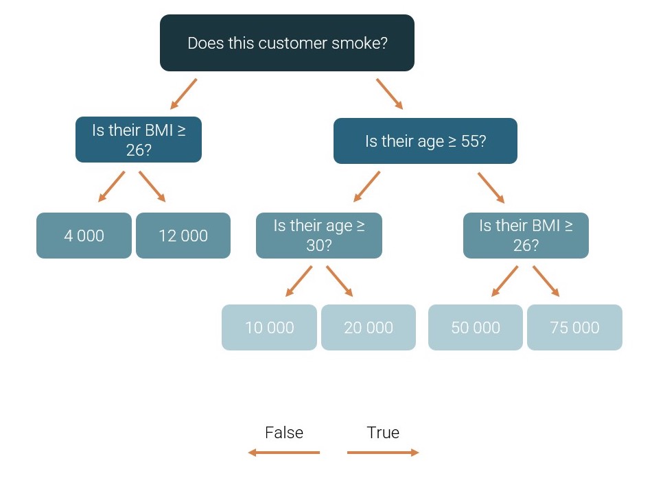
Figure 2: A simple decision tree predicting insurance costs

If you answer a question in the affirmative, you go to the right and answer the next question. Otherwise, you go to the left. When you reach a blue box (a ‘leaf’ of the tree), that value becomes your predicted insurance cost. For example, a smoking customer aged 60 with a BMI of 24 would get a predicted insurance cost of 50 000.

Note that, in addition to BMI and age, we use information about whether the customer smokes to make our predictions. This ‘smoking status’ is a Boolean variable, i.e. a dimension. One of the benefits of decision trees as compared to a more conventional mathematical expression is that they can handle both measures and dimensions as influencer variables.

The graph of a decision tree will not be a smooth curve like the one in figure 1(b), but rather a ‘jagged’ set of planes. I would like to show you the graph of the decision tree in figure 2 as an example, but I cannot display the graph if our prediction uses more than two inputs. Let us therefore limit ourselves to the right subtree of the decision tree in figure 2; its graph is displayed in figure 3(a):

Figure 3(a)                                                  Figure 3(b)

We can also produce a top-down view and use color to indicate the target value (figure 3(b)); this highlights the fact that a decision tree essentially splits the input space into several subspaces and assigns an estimated target value to each of them.

Finding the Best Decision Tree

Let me start by defining exactly how we measure how ‘good’ or ‘bad’ a decision tree is, so that we can quantify what the ‘best’ tree is. We introduce a loss-function, which measures the overall error a tree f commits:

The idea, in short, is that we calculate the error (f(x_i) – y_i) the tree commits in each training example, square it, and sum over all training examples. The motivation for squaring the error is in part that it ensures negative errors also count positively, and in part that large errors are punished much more heavily than small errors.

The error f(x_i) – y_i is also known as a ‘residual’, so the above loss function is commonly known as the residual sum of squares (RSS).

Our goal will be to minimize the RSS. We need to determine which questions to ask, and what target values to assign to each leaf. The possible questions that can be asked are:

• For dimensions: Assume the dimensions can take on K different values. We then have K possible questions to ask: ‘Does this dimension have the first possible value?’, ‘Does it have the second possible value?’, etc.
• For measures: There may be an infinite number of possible values for a measure, but within the training data set it will only take on a finite number of values. Call these values v₁, v₂, …, v_K. The possible questions we will consider are then ‘is the value greater than (or equal) to v₁?’, ‘is it greater than (or equal) to v₂’ etc.

The algorithm we will use to (hopefully) minimize the RSS is a greedy algorithm which finds one new question to ask at a time. It starts off with an empty tree, chooses the ‘best’ question to ask, and then repeats the process on each of the created subbranches. More formally:

1. Make a list of every possible question according to the description above. For every possible question:
   • Try asking the question of every training example.
   • Calculate the average target value of the training examples that end up in either branch.
   • Use these averages as the tree’s predictions for either branch.
   • Calculate the loss of the tree if this question is used.
2. Extract the question which gives the smallest loss and add this question to the tree.
3. Recursively repeat step 1-3 on each of the created subtrees (including only the questions that are relevant for the training examples that go there) until the tree reaches a certain maximal depth or the loss becomes sufficiently small.

It can easily be shown that using the average target value of the training examples in a given leaf as that leaf’s prediction, will minimize the loss value (the mathematically inclined might try differentiating the RSS w.r.t. a constant function value f(x) = c, and setting the derivative equal to zero).

The process is visualized in the video below, in which I have returned to the example of predicting insurance costs from a customer’s BMI and age. In the top right, we see the tree growing one question at a time, and each time a new question is added, we see the target value estimates we would have used if we stopped growing the tree at that point.

Only the first 4 nodes in the tree are determined in the video, but in practice, we could of course continue the process for much longer.

Gradient Boosting: Combining Decision Trees to Avoid Overfitting

In the previous section, I elegantly avoided the question of how to select the maximal depth of a decision tree.

If we constrain the maximal depth a lot, our tree will only be able to divide the input space into a few subspaces, and the tree will therefore not be able to describe the output very precisely (in figure 2, for example, we can only guess 6 different values, so if a customer’s ‘correct’ insurance cost was 35 000, we would never be able to predict it accurately).

On the other hand, if we allow our tree to grow very deep, we obtain exponentially more possible target value estimates, and it is not at all unlikely that we will be able to make a function that predicts the target value with 100% precision on the training data (we just need to split the input space into as many subspaces as there are training data points). But if we do this, our model will be very prone to what is known as overfitting. Simply put, a model is overfitting if it performs very well on the training data, but its predictions don’t generalize well to new data (which is what we’re really interested in). Overfitting usually occurs when we train a very complex model (i.e. one with many parameters, such as a deep decision tree) on a limited amount of training data; the model can simply ‘memorize’ the training examples rather than find the true relationship between the influencer variables and the target value, as illustrated in figure 4.

Figure 4. The true function from which the data is generated (with a bit of noise) is the dark blue line. We try fitting polynomials of varying degrees (i.e. models of varying complexity) to the data points. If the model is too complex (light blue curve), it will fit the data points perfectly, but will not be very close to the true function.

To avoid overfitting, while still being able to describe the potentially complex relationships in the data, SAC Smart Predict makes use of an algorithm known as Gradient Boosting. The idea is to use the combined outputs from an ensemble of shallow decision trees to make our predictions –individually, they are so simple that they couldn’t possibly overfit, yet when their efforts combine, they are able to describe complex relationships.

Figure 5. Combining decision trees to avoid overfitting

Let K denote the maximal number of simple decision trees that we will combine.

The algorithm proceeds as follows:

1. Start with the simplest decision tree imaginable, which will simply output a constant value no matter what input it receives. Let us call this decision tree f₀. At this point, our final regression function is just f = f₀.
2. For k from 1 to K:
   1. Calculate the error that f commits in every training data point: e_i = f(x_i) – y_i.
   2. If the loss (i.e. the sum of squared errors) is sufficiently small:
      • Break out of the loop.
   3. Otherwise:
      • Determine a decision tree f_k of maximal depth 4 to predict the error e_i as a function of x_i.
      • Update f = f + λf_k, where λ is a small constant (usually set to fx. 0.1).

Note that, even though f_k is used to predict the errors that f commits, we do not just add it to the previous f, we multiply it by a small constant first. This helps smooth out the final f, further avoiding overfitting (but also means that we will have to include a larger number of decision trees to describe the training data).

In Conclusion

SAC Smart Predict is a powerful tool in the planning toolbox, and perhaps its most important quality is the incredible ease with which even non-technical users can create predictive models with just the click of a button. Still, it doesn’t hurt to peek into the black box and understand the inner workings of the algorithms in use. My hope is that this blog post has helped you do just that and helps to demystify the results of any future regression models you may train.