understanding classification with smart predict
In this blog post, I will explain the machine learning algorithms underlying classification in SAC Smart Predict. The focus will be on building the theoretical framework necessary to truly understand the output produced within SAP Analytics Cloud.
Martin Bregninge’s previous post, ‘Understanding Regression with Smart Predict‘, shares many similarities with this one, but we have intentionally written both posts to be read and understood independently of the other. If you have already read the regression-post, many of the concepts discussed here will be familiar to you already.
I have included small boxes like this one, describing sections that can be skipped, and providing additional insight by comparing classification to regression.
The Point of Classification
This section should not be skipped. Note that the setup for classification is the same as regression, except that our target value is a binary dimension instead of a measure.
Classification is the task of sorting objects into categories (or classes), based on the known values of some influencer variables that describe the objects. For example, classification can help us answer such questions as:
- “Is this employee in danger of leaving the company?”
- “Is this item from our manufacturing plant faulty?”
- “Is this potential customer going to be interested in our services and thus receptive to our marketing?”
Influencer variables can be both dimensions (nominal variables such as the gender of a potential customer) and measures (numerical variables such as the temperature at which an item was manufactured). The target value must be a dimension, and each possible member of the dimension corresponds to a different category that the object can belong to.
You might notice that all the examples I’ve given are ‘yes/no’-questions – in other words, the target value can only take on two distinct values, such as ‘faulty’ or ‘not faulty’.
I have limited myself to these examples because the algorithm used by SAC Smart Predict performs binary classification; we cannot sort objects into more than two categories. Serious as this limitation may seem, it has its benefits. For one, it allows us to easily estimate the probability of belonging to each category (we’ll see how in a minute!) rather than just giving a deterministic classification. If we wish to classify many objects, we can thus sort them in order of probability, allowing us to reformulate our questions slightly:
- “Which of our employees are most likely to leave the company?”
- “Which items from our manufacturing plant are most likely to be faulty?”
- “Which potential customers are most likely to be receptive of our marketing?”
The Idea Behind Classification
This section can be skipped. In short: We will try to find a function which gives the probability that a certain input belongs to class 1 rather than class 0. Our final classification is based on this probability. Figure 2 illustrates how the classification problem can be reframed as a regression problem.
Throughout this blog post, I will return to the example of using influencer variables age and income to predict which potential customers are most likely to be receptive to our marketing.
To make our predictions, we will need a large set of labeled training data: people for which we know the influencer variables, and whether they are marketing-receptive or not. We might plot our training data as shown in figure 1(a).
Our goal will be to determine a function, f, which – given the age and income of a person – outputs an estimate of the probability that this person is marketing-receptive. For our toy dataset, one possible function is shown by the background color in figure 1(b). It should be clear for us as humans that this is a reasonable choice of the probability function. In the section on Maximum Likelihood, we will define formally what constitutes the ‘best’ choice, so that a computer can understand it.
For now, just note that (almost) all the marketing-receptive customers are predicted to be likely to be marketing-receptive, and similarly for the unreceptive customers. The model lines up well with reality, so it seems reasonable to expect that it will also make good predictions in new cases.
From the probability function, we can create a decision boundary (the black lines in figure 1(b)) which is used to perform the final classification. The decision is made by asking if the probability of being class 1 is above some threshold (in this case 50%).
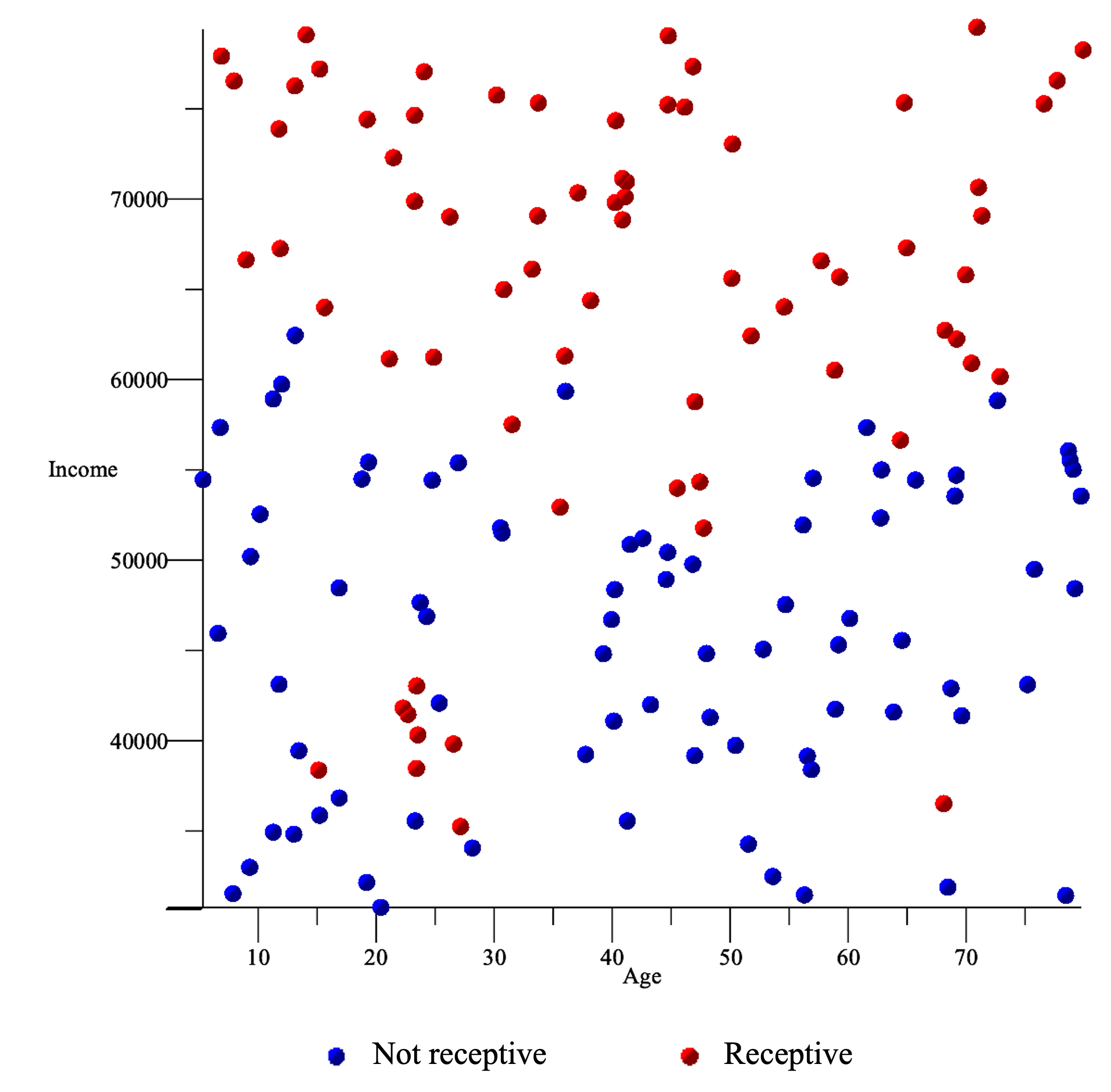
Figure 1(a): Our training dataset contains 150 people. We know their age, their monthly income, and whether they are marketing-receptive customers or not.
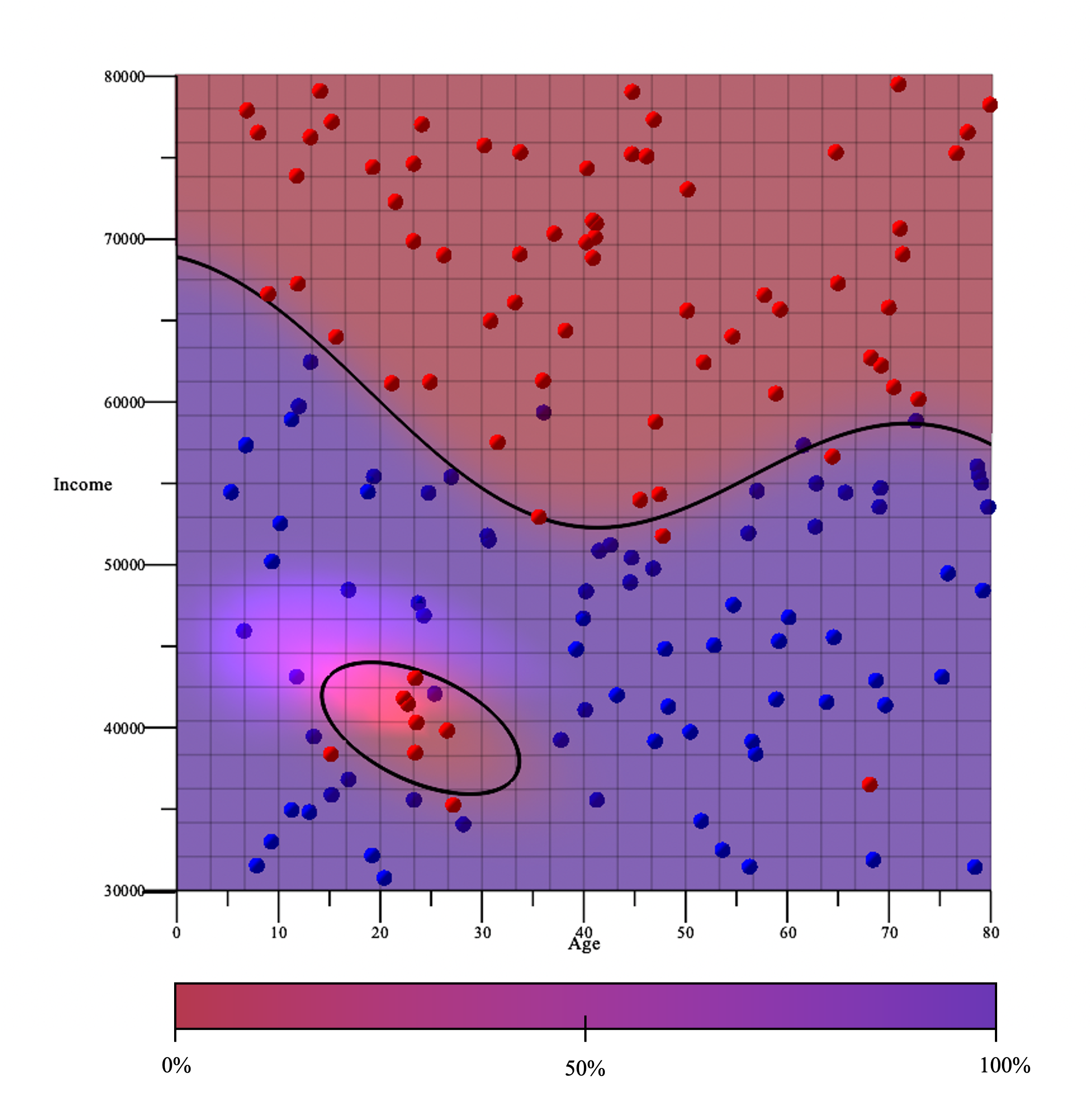
Figure 1(b): A reasonable probability function and decision boundary. We will predict customers to be receptive if they are within one of the red areas. Note that not every point is correctly classified – that won’t always be possible.
Instead of using the background color to represent the probability f(x) (as in figure 1(b)), we could use a third axis, as shown in figure 2. We also group the training examples along the new axis according to their target value (encoded either as a 0 or 1, since there are only two possible target values).
For those familiar with regression, this visualization should make it clear that the regression framework is directly applicable. The only difference to simple regression, as we will see shortly, is that we can improve our loss function somewhat, because we want to interpret f as a probability function.
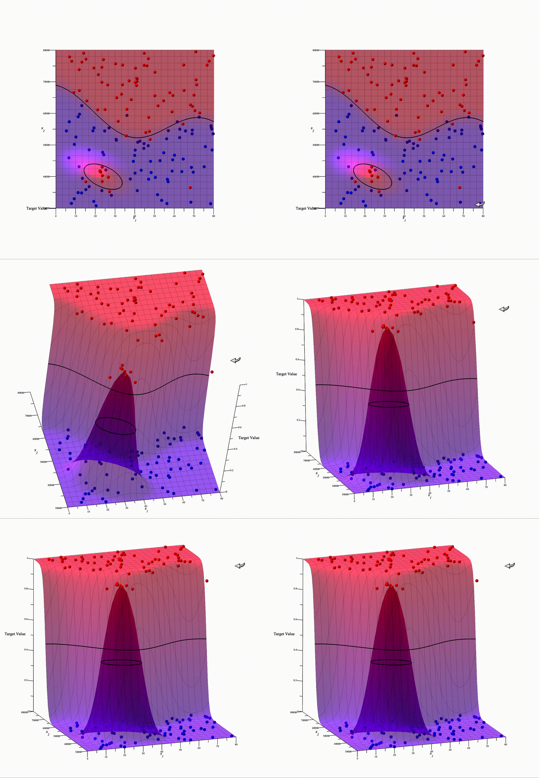
Figure 2: Each training data point consists of two influencer variable values and a target category. By assigning a number to each category (either 0 or 1) we can represent the points in three dimensions, and our desired probability function should look similar to the one in the figure.
Finding f
This section should not be skipped.
Let’s try to formalize and generalize our setup: We will store the influencer variables of the i’th training example in a vector, xi, and we will encode the corresponding target value in a binary variable, yi. For example, we could have yi = 1 corresponding to a marketing-receptive customer and yi = 0 corresponding to the opposite.
There are two important questions to answer to find a good probability function f:
- What type of function should it be?
- How do we find a good function of this type?
What f should look like: Decision Trees and the Logistic Sigmoid
Since Smart Predict is meant to work for almost any dataset, we want the function type to have a lot of flexibility, so that it can describe very different relationships between input and output. This flexibility is provided by using a decision tree (explained below). We also want to ensure that the final output is a number between 0 and 1, so we run the decision tree’s output through a logistic sigmoid function (see figure 3).
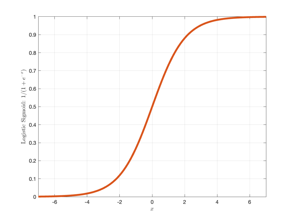
Figure 3: The graph of the logistic sigmoid, σ(x) = 1/(1+exp(x)). It squeezes all the real numbers into the range between 0 and 1, while still retaining all the information, because it is an invertible function.
If you’ve ever heard of logistic regression, this idea of running a flexible function – in that case, a standard linear model – through a logistic sigmoid should be familiar.
The rest of this section is skippable.
But in our case, we use a decision tree instead of a standard linear model. A decision tree essentially asks a series of questions of its input and gives an output depending on the answers. The decision tree makes no prior assumptions about the relationships we want to describe, and it can handle both dimensions and measures as input. A very simple decision tree (followed by the logistic sigmoid) that tries to determine if a customer is marketing-receptive could look like this:
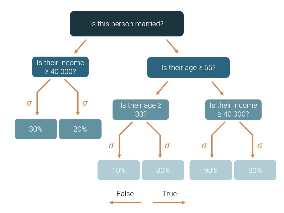
Figure 4: A decision tree (followed by a logistic sigmoid, σ) which tries to determine if a given person is marketing-receptive. For example, the model is 90% confident that a married person of age 60 with an income of 30 000 is receptive. It only thinks there’s a 20% chance that a non-married person with an income of 50 000 is receptive, so it is 80% confident that such a person is not receptive.
In each ‘leaf’, the decision tree guesses on a constant value – the same for every input that ends in that leaf – which is then run through the logistic sigmoid.
Maximum Likelihood: Defining what constitutes a ‘good’ model
This section should not be skipped.
We need to define a measure of how ‘good’ or ‘bad’ a given model is, so that we can find the best one.
Recall that we used the Residual Sum of Squares as our Loss function for regression, and we wanted to minimize it, because it measured how ‘bad’ our model was; in the case of classification, we have a slightly more complex expression, and we want to maximize it, but the approach is the same.
We stated in the beginning that we want the predicted probabilities on all the training examples to match up well with the true category. In other words, the probability of the actual observations according to the model should be as large as possible. Let’s unpack what this means:
If f(xi) = 0.9, then the model predicts that there’s a 90% chance that example i is category 1, and a 10% chance it is category 0.
Therefore, if the actual value of yi is 1, the probability of that is 90% according to the model. On the other hand, if yi = 0, the probability of the actual observation according to the model is just 10%.
We can write this as

in which P(yi | f) should be read ‘the probability of the actual observation, yi, given that the model, f, is correct’. The second equality is true since lifting to the 0’th power makes any number into 1 (you can easily check that the two sides of the equality sign are the same in each of the cases yi = 0 and yi = 1).
By multiplying these probabilities from every point, we get the probability of all the observations given the model. Our final goal is thus to maximize

where n is the number of training examples.
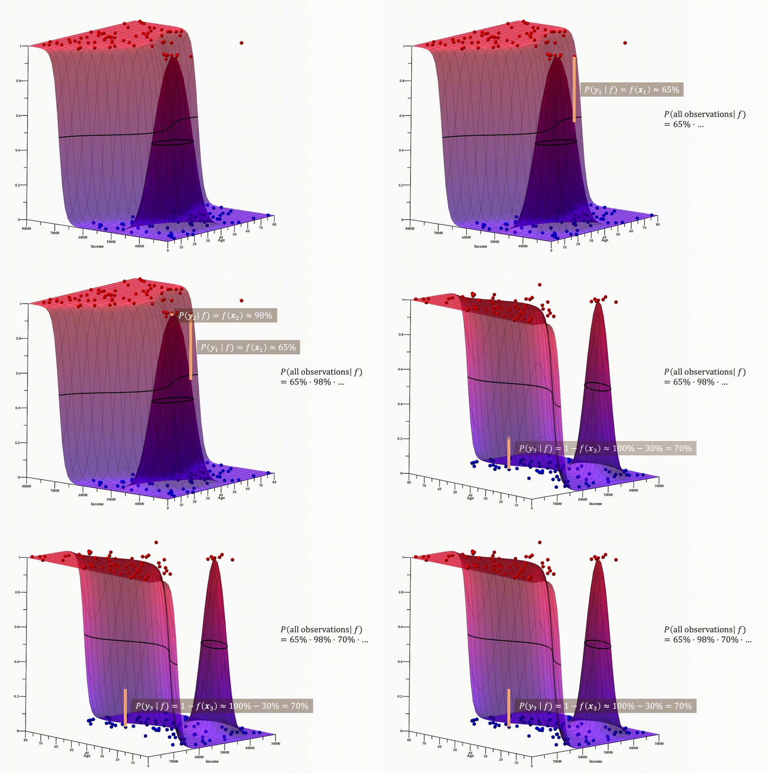
Figure 5: The probability of the observations given the model is calculated by evaluating the function in each point and multiplying the resulting probabilities.
The above explains everything important about the idea of Maximum Likelihood estimation: We want to find the function that maximizes the probability of the observed data, which is given by equation (1). There’s still quite a bit of math to work through before we can find this function – it will be described in the appendix, but it requires that you have read the sections on finding the best decision tree and Gradient Boosting first.
Finding the best decision tree according to Maximum Likelihood
This section is the same as in the regression blog post, except that we use the new loss-function.
We need to determine which questions to ask in the decision tree, and what probabilities to assign to each leaf. The possible questions that can be asked are:
- For dimensions: Assume the dimensions can take on K different values. We then have K possible questions to ask: ‘Does this dimension have the first possible value?’, ‘Does it have the second possible value?’, etc.
- For measures: There may be an infinite number of possible values for a measure, but within the training data set it will only take on a finite number of values. Call these values v1, v2, …, vK. The possible questions we will consider are then ‘is the value greater than (or equal) to v1?’, ‘is it greater than (or equal) to v2’ etc.
The algorithm we will use to (hopefully) maximize formula (1) is a greedy algorithm which finds one new question to ask at a time. It starts off with an empty tree, chooses the ‘best’ question to ask, and then repeats the process on each of the created subbranches.
More formally:
- Make a list of every possible question according to the description above. For every possible question:
- Try asking the question of every training example and split the examples into a ‘yes’ and a ‘no’-group, thus creating two new provisional leaves in the tree.
- Determine the best constant value to use as the tree’s prediction in each leaf (this part is also relegated the appendix, since it requires diving into the nitty-gritty mathematics).
- Calculate the total loss of the tree if this question and these constant values are used.
- Extract the question which gives the smallest loss and add this question to the tree.
- Recursively repeat step 1-3 on each of the created subtrees (including only the questions that are relevant for the training examples that go there) until the tree reaches a certain maximal depth or the loss becomes sufficiently small.
For the regression blog-post, we produced a little video illustrating the algorithm for finding the best decision tree (in a regression context). It still makes sense for classification – just imagine that the z-axis is limited between 0 and 1.
Gradient boosting: Combining decision trees to avoid overfitting
This section is almost exactly the same as in the regression blog post and can safely be skipped. You might want to consider figure 6.
In the previous section, I elegantly avoided the question of how to select the maximal depth of a decision tree.
If we constrain the maximal depth a lot, our tree will only be able to divide the input space into a few subspaces and might not be able to describe the output very precisely (in figure 4, for example, we can only split the population into 6 different groups).
On the other hand, if we allow our tree to grow very deep – potentially splitting the input space into as many subspaces as there are training data points – we can obtain 100% accuracy on the training data. But if we do this, our model will be very prone to what is known as overfitting. Simply put, a model is overfitting if it performs very well on the training data, but its predictions don’t generalize well to new data (which is what we’re really interested in). Overfitting usually occurs when we train a very complex model (i.e., one with many parameters, such as a deep decision tree) on a limited amount of training data; the model can simply ‘memorize’ the training examples rather than find the true relationship between the influencer variables and the target value, as illustrated in figure 6.
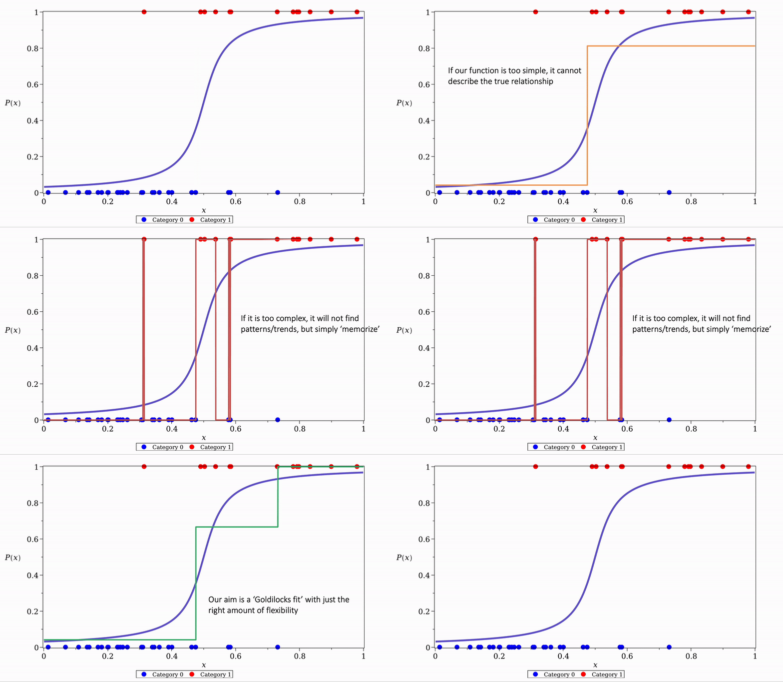
Figure 6. Attempting to fit decision trees of varying complexity to a simple classification problem with just one influencer variable, x.
The blue curve describes the true probability that a certain object is category 1 given a known x-value. As such, the graph of our decision tree should match it as closely as possible. The red and blue dots are the training examples.
It is clear that the red curve – made by allowing the decision tree to split the input range 20 times – fits the training data very well but won’t generalize as well to new data as the simpler models.
To avoid overfitting, while still being able to describe the potentially complex relationships in the data, SAC Smart Predict makes use of an algorithm known as Gradient Boosting. The idea is to use the combined outputs from an ensemble of shallow decision trees to make our predictions –individually, they are so simple that they couldn’t possibly overfit, yet when their efforts combine, they are able to describe complex relationships.

Figure 7. Combining decision trees to avoid overfitting
It starts with the simplest imaginable decision tree – which simply outputs a constant value regardless of its input. We then calculate the error committed by this first tree in every training example, and train a new, small decision tree to minimize the error when it is added to the first. This process is repeated until the error becomes sufficiently small or a maximum number of trees is reached.
From probability to classification
As nice as it is to know that a certain customer is 75% likely to be marketing-receptive, there are many applications in which we will need to perform a final clear-cut classification of our objects.
This is a relatively simple task once the probability function, f, has been determined. We simply choose some threshold and classify a new object, xnew, as being category 1 if f(xnew) is above this threshold. In figure 1(b), I used 50% as the threshold to draw the decision boundary. This is of course a natural choice, but in some cases, we might prefer different thresholds. If, fx., we have 20000 potential customers and the capacity to market towards 2000 of them, we would just choose the 2000 that were most likely to be marketing-receptive (which could just as well correspond to a threshold at 25% or 75%). This form of thresholding is quite common, and in the Smart Predict interface, it is controlled by the ‘Contacted population’ slider.

In conclusion
As I have attempted to illustrate, the key ideas needed to understand classification are almost exactly the same as the ones needed to understand regression. In a sense, for a reader who understands regression, this entire blog post can be summarized by figure 5. Everything else is just technicalities!
If you learned something new from this blog post, follow Innologic on LinkedIn in order to stay up to date on our latest Business Intelligence and Analytics content.
Written by the Innologic SAC Team
Appendix
Maximizing the product from formula (1) is the same as maximizing the logarithm of the product, which can be rewritten as follows:

The reason that we make this reformulation is that computers generally have an easier time summing small positive numbers than multiplying them without making errors.
We usually formulate optimization problems as minimization problems, so we add a minus to the above expression and obtain a loss function:

EXPRESSION 1
When doing classification, it is a somewhat arbitrary choice which class should be ‘category 0’, and which should be ‘category 1’, so we would like our algorithm to produce the same results regardless of the choice. We will rewrite the expression above a bit more to ensure this symmetry.
If we have a certain probability, p, of belonging to category 1, the probability of being category 0 is of course q = 1 – p. The associated odds are defined as the number p/q, which is between 0 and infinity. We also commonly speak of the log odds, log(p/q), which can be any real number. Taking the logarithm of the odds gives the nice symmetry we want, since common logarithm rules yield:

This means switching the categories simply corresponds to adding a minus to the log odds, and this turns out the be unimportant for the decision tree algorithm we will use.
Because the log odds have this favorable quality, we will not actually attempt to find the probability function f as a decision tree; instead, we will attempt to find a decision tree, g, which predicts the log odds, and only afterwards use the log odds estimate to calculate the probability.
Note that that if g is the log odds of f, i.e. if

we can isolate f as:
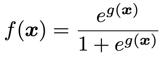
Substituting this into expression 1 – since our ultimate goal is still to find a maximum likelihood-function – yields

Now note that

while

Plugging these results back into Loss(g) gives

This, finally, is the loss function we will use.
Now for the actual optimization algorithm. Like I mentioned earlier, the ‘best’ decision tree is found using a greedy algorithm, which
- starts with an empty tree
- asks every possible question of the input data
- for each question, determines the best constant values to use in either provisional leaf and calculates the resulting loss
- picks the question which gives the lowest loss, and repeats the process on both of the created subbranches
The central step, which I glossed over in the main text, is determining the best constant value to use in each leaf when testing a certain question. The process is complicated further by our choice to use gradient boosting, since different training examples might end up in different leaves in different trees.
Let’s start by ignoring the gradient boosting, and considering the very first tree, g0, which should simply output a constant value regardless of the input.
For regression, when the loss function was the residual sum of squares (RSS), the best constant value was just the average of the target values in a certain leaf. This makes a lot of sense intuitively but could also be explained formally by calculating the derivative of the RSS w.r.t. the constant value, setting it equal to zero, and solving for the constant value. We will apply the same method to the new loss function here.
In this first tree, g0(xi) will be equal to a constant c no matter which i we are looking at, so we can express the loss purely as a function of c:

in which k is the number of elements of category 1 (since yi will be 1 in exactly k elements of the sum).
To minimize this, we take its derivative with respect to c and set it equal to zero:
Assuming k ≠ n this yields:


Recognize that k/n is the probability of a random example being category 1. In other words, c is simply the log odds of such an example being category 1.
Now assume that we have found m trees – g0, g1, …, gm – and we have combined them into a total tree, g. The next step is to find gm+1 such that g + gm+1 minimizes the loss. When we are testing out a certain question, we must pick a constant value in each of the provisional leaves. Since the loss function is a sum, the choice of constant value in one leaf does not affect what value should be chosen in the other leaf. Let us therefore limit ourselves to considering a single leaf. Assume that the objects xi for i ∈ I (where I is some index set) are the ones that end up in this leaf. If gm+1 uses the constant value c as our prediction in the leaf, the final prediction of the log odds will be given by g(xi) + c, so the contribution from the leaf to the loss function is:

To pick the best c, we could take the derivative and set it equal to zero as before, but due to the complexity of the expression above (note that g(xi) may be different for different i’s, since the training examples may have ended up in different leaves in previous trees), that is easier said than done. We will therefore derive the second-order Taylor polynomial approximation to the expression, calculate its derivative, and set that equal to 0.
The second-order Taylor polynomial at c = 0 is

and its derivative is

Setting it equal to 0 and solving for c yields
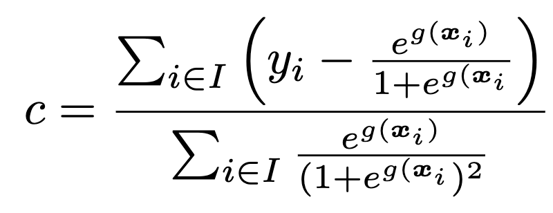
When we’re trying to determine gm+1, every part of this expression is known, so it is simply a matter of evaluating it.
This concludes the discussion of the mathematics required to implement gradient boosting for classification.
